Smoothed-Particle Hydrodynamics
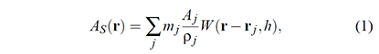
Smoothed Particle Hydrodynamics (SPH) is a computational technique for simulating fluid behavior. It represents a fluid as a collection of particles, where each particle carries properties like position, velocity, density, and pressure. SPH is an interpolation method for particle systems. According to SPH, a scalar quantity A is interpolated at localtion r by a weighted sum of contributions from all particles:
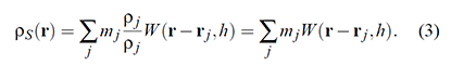
SPH calculates densities by summing the contributions of nearby particles using a smoothing kernel within a defined smooth radius. The "smooth radius" determines the range of influence for each particle, allowing SPH to capture complex fluid interactions like splashing and turbulence while simulating fluids like water or air. A smoothing kernel in the context of Smoothed Particle Hydrodynamics (SPH) is a mathematical function used to calculate weighted contributions from neighboring particles within a specified radius. The kernel function assigns higher weights to particles closer to the target and lower weights to those farther away, ensuring that contributions smoothly taper off with distance.
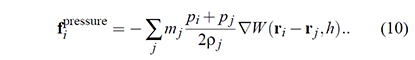
Pressure forces arise from the difference between the calculated density and a target density, enforcing fluid compression and expansion. Pressure forces push particles apart when the density is higher than a specified target density and pull them together when it's lower. High-pressure regions result in areas of compression, while low-pressure regions lead to expansion, creating fluid motion and behaviors like fluid movement and surface tension.
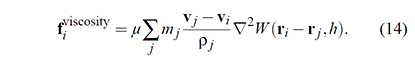
Viscosity is simulated by applying forces based on the relative velocities of neighboring particles. Viscosity forces help capture effects like fluid stickiness and internal friction. When neighboring particles have different velocities, viscosity forces act to equalize their velocities, which results in the smoothing out of fluid motion.
Thus, the steps for calculate the position for each particle at each move would be
For each particle i in the list:
1. Calculate the predicted velocity and position by applying the gravity and other external forces.
2. Loop all particles to update density by applying the density equation with smooth kernle.
3. Use updated density value to calculate pressure force.
4. Update viscocity using the velocity value.
5. Update particle position.

Grid-based Spatial Index Structure
The above steps through the entire particle list to calculate which particles will contribute density and pressure force to each sample point. However, this brute-force approach resulted in significant time wastage as searching for valid neighboring particles.
One promising approach to optimize this process is the implementation of a Grid-based Spatial Index structure since the property contribution only care about the particles that reside inside of the smooth radius circle which centered at the given sample point. This structure employs a non-fixed size grid system, meaning that it dynamically adapts to the number of particles within the space without requiring predefined dimensions. Here's how to contrcut the Grid-based spatial index structure:
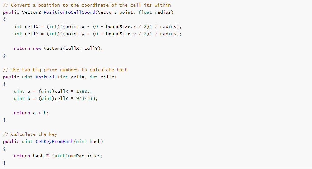
1. Obtain cell coordinates based on each particle's location within the space.
2. Calculate a hash value for the cell coordinates.
3. Use the modulus operation with the size of the particle list to determine the key value for the given particle.
2. Calculate a hash value for the cell coordinates.
3. Use the modulus operation with the size of the particle list to determine the key value for the given particle.
To facilitate spatial index searches, these three arrays are needed:
1. Particle Index Array: This array stores the indices of particles in the particle list.
2. Particle Cell Index Array: Each element in this array contains the hashed cell coordinate for the corresponding particle in the Particle Index Array.
3. Hash Start Index Array: In this array, the indices correspond to hash values, and the values at each index indicate the starting index within the sorted Particle Cell Index Array.
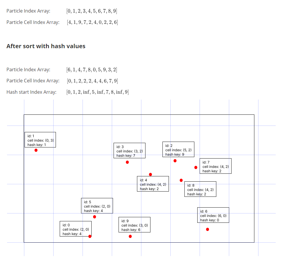
Following the movement of particles, our next step involves updating the three arrays mentioned above and ensuring that both the Particle Index Array and Particle Cell Index Array are sorted.
1. Calculate the Cell Coordinate: For each sampled particle, examine a 3x3 grid centered at the cell of the sample particle, as the size of each grid corresponds to the smooth radius. To find the cell coordinates of neighboring grids, simply add offsets to the sample particle's cell coordinates.
2. Calculate the Hash Value: With the cell coordinates of the neighboring grids in hand, apply the hash function to each set of coordinates to calculate a key value for each grid.
3. Locate Start Index: As the Particle Index Array and Particle Cell Index Array have been sorted, use the Hash Value Array to locate the start index corresponding to the key value of the current grid. This index is essential for identifying the starting point of particles with the same hash keys.
4. Identify Particles: By utilizing the Hash Start Index Array, one can pinpoint the starting position for the current hash value. This enables us to access all particles that share the same hash key.
5. Validate Neighbors: It's important to note that due to potential hash collisions, not all particles sharing the same hash key will necessarily be within the smooth radius circle of the sample particle. Therefore, additional validation is required.
By systematically following these steps, each particle can locate and validate neighboring particles within its smooth radius circle. This process optimizes the computation of densities and pressure forces in our simulation, enhancing its overall efficiency and accuracy.
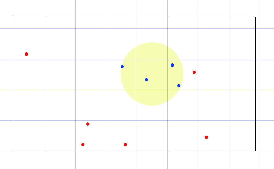
The following images illustrate how grid-based spatial searching operates in both 2D and 3D fluid simulations, ultimately achieving results equivalent to looping through all particles within the space.
2D Grid-based spatial searching
3D Grid-based spatial searching

Compute Shader and GPU Instancing
While the grid-based spatial index structure significantly reduces the time spent searching for neighboring particles to calculate density and other physical fields, it is essential to address the issue of high running times, primarily attributed to CPU-side computations. Additionally, the presence of a large number of particles necessitates a substantial number of draw calls, further impacting overall performance. To mitigate these challenges, two advanced techniques, namely Compute Shader and GPU Instancing, are introduced to the project. These techniques utilize the parallel computation capabilities of the GPU, resulting in a substantial enhancement in performance.
The Compute Shader leverages General-Purpose computing on the GPU. Given that fluid simulation entails the computation of physical properties for each individual particle, harnessing the parallel computational power of the GPU becomes invaluable. This approach significantly accelerates the simulation process compared to using the CPU for calculations.
GPU Instancing is able to simulate multiple instances sharing the same mesh within a single draw call. Given that particles in the scene are all based on the same mesh, employing a buffer to modify instance vertex positions within the vertex shader emerges as an optimal choice, resulting in substantial time savings.

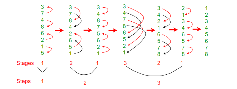
GPU Sorting Algorithm
Currently, all calculations related to physical properties are executed on the GPU, resulting in consistent frame rates, even when dealing with a substantial quantity of particles within the scene. Furthermore, the optimization of performance is achieved through the utilization of a grid-based spatial indexing structure on the GPU. The key point of spatial structure is that the entire list need to be sorted based on the hash value. On GPU side, in order to maximize the potential of parallel computing capabilities, the Bitonic Sort algorithm emerges as the most fitting choice when implemented on the GPU.
Bitonic Sort established from the key concept Bitnoic Sequence, which is a sequence that exist an index i for which all elements less than or equal to i are in increasing order, and all elements greater than or equal to i are in decreasing order and vice versa. Moreover, Bitonic Sort is able to leverage the parallel computing since it always compare elements in a predefined sequence and the sequence of comparison doesn’t depend on data.

Further Works and references
There are multiple potential works to continue optimize the fluid simulation. One is that using Ray Marching to simulate the fluid volumn. Another optimization work is to add external force so that particles can have interaction with different objects.
Reference about this project:
https://sph-tutorial.physics-simulation.org/pdf/SPH_Tutorial.pdf
https://matthias-research.github.io/pages/publications/sca03.pdf
https://web.archive.org/web/20140725014123/https://docs.nvidia.com/cuda/samples/5_Simulations/particles/doc/particles.pdf
https://www.geeksforgeeks.org/bitonic-sort/
https://www.youtube.com/watch?v=rSKMYc1CQHE&t=1692s